
But what if the numbers we use every day are not the only possible number system? In today’s article, we will explore this question and endeavour a mathematical excursion into the world of p-adic numbers.
i) Building the numbers we know
In this previous article, Jort de Groot already explained in detail how to construct the real numbers that we know. Have a look there if you want all the details, to keep the present article self-contained, I will also give a quick review of the construction here.
Let’s take the simplest imaginable number as our starting point: 1. Using only the operation of addition, we can use 1 as a “building block” to build all positive whole numbers, also known as the natural numbers:
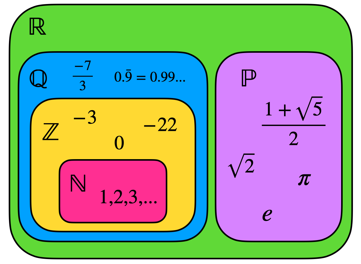
\( \huge \mathbb{N}=\{1,2,3,4,\ldots\}. \)
If we also want to make the operation of addition reversible, by introducing subtraction, we however soon run into a problem. For instance, what should the number 3 − 5 be? To make sure that subtraction is always possible, we need to introduce negative numbers and zero, by which we obtain the set of the integers:
\( \huge \mathbb{Z}=\{\ldots ,-2,-1,0,1,2, \ldots \}. \)
We can moreover introduce another familiar operation: multiplication. If we also make sure that we can reverse that operation, by dividing numbers, we can use the integers to construct an even bigger set of numbers, known as the rational numbers (or just the rationals). The rationals are then all those numbers which can be defined by simple fractions, i.e. under the form p/q where p and q are both integers (and q is non-zero). Note that, in fact, every integer is already a rational number, since we can write, for example, 5 as 5/1. Thus, we can say that the set of integers is contained in the rationals. It is difficult (though not impossible!) to write these rationals as a nicely ordered set as we did for the natural numbers or the integers, so let me just give some examples:
\( \huge \mathbb{Q}=\{\ldots,-2/1,-1/2,0,3/7,5/6,\ldots\} \)
An important realisation is that every rational number can alternatively be written as a decimal expansion, i.e., ⅓ = 0.3333…, that either ends after finitely many digits or eventually repeats. In a sense, the rational numbers can thus be viewed as a discrete collection of points on the number line.
However, the real numbers are an infinitely bigger set than only the rationals, because there are many more numbers “in between” the fractions defining the rationals, as explained in Jort’s previous article. For instance, it can be shown that no fraction can equal exactly √2. No matter how hard you try, there are no integers p and q such that p/q equals √2.
Numbers like √2 are called irrational numbers; they have decimal expansions that continue forever without ever settling into a repeating pattern. Other famous examples include π, the ratio between a circle’s circumference and diameter; Euler’s number e, which appears throughout calculus and growth processes, or the golden ratio (1+√5)/2.
Together, the rational and irrational numbers form the real numbers. The real numbers can be visualized as the entire number line without any gaps, producing a continuous number system.
ii) Real numbers are a completion of the rationals
The idea of “filling the gaps” turns out to be an extremely important concept in the mathematics of numbers. Mathematicians formalize this process by saying that the real numbers are a completion of the rational numbers, meaning that all the “missing points” needed to make the discrete rational number line continuous have been added.
How can we then implement such a completion? Suppose we want to approximate an irrational number, like √2. We can do this by writing a sequence of rational numbers that get closer and closer to its true value, for instance: 1.4, 1.41, 1.414, 1.4142, …
You can see that each term in this series, while still being a rational number (for example, 1.41 = 141/100), improves upon the previous one and gets closer (or in mathematical language: converges) to the actual value of √2. However, even though the sequence gets ever closer to a definite number, its limit is not rational because the digits behind the decimal will never terminate or start to repeat. In the limit of infinitely many decimals, the approximation thus lies outside the set of rational numbers.
This reveals a weakness of the rational numbers: some perfectly reasonable sequences do not converge to a rational number. To fix this problem, mathematicians enlarge the rationals by adding all the missing limits, which produces the set of real numbers by a process called completion. In a sense, the real numbers are thus what you obtain when you take the rational numbers as your starting point and then “fill in all the holes between them”.
iii) Distance matters!
At first glance, this seems like the end of the story. (You might have heard of complex numbers before, but we will skip those in today’s discussion.) There is however an important question regarding completion: What do we actually mean when we say that two numbers are “close”, or that a limit series gets closer and closer to the actual value of an irrational number?
Usually, we measure distances using the ordinary absolute values of numbers, denoted |x| in mathematics. Two numbers are then considered close if their numerical difference is small. For example, 100 is much closer to 101 than to 1000, since the first difference, 1, is much smaller in absolute value than the second distance, 900. Similarly, 0.001 is much closer to 0 than it is to 10. This definition of distance feels natural to us because it matches our everyday experience of physical space: a one-meter step is much smaller than a nine-hundred-meter walk. As a result, we instinctively think of numbers as being arranged along a line, or a ruler, and we judge how close they are by looking at how far apart they sit on that ruler.
As stated before, the rational numbers can be thought of as the markings on such a ruler. However, between any two markings we can always add more and, even when we do so, there are still tiny gaps corresponding to irrational numbers such as √2 or π. All of the real numbers can then be obtained by filling in all the gaps, turning the ruler into a completely continuous line.
But mathematicians have wondered: what if the ruler itself were not unique? What if there were a different, but equally valid, way of measuring distances? As it turns out, if we change our notion of distance, we can obtain a completely different completion of the rational numbers. That idea leads us to the p-adic numbers.
iv) p-adic numbers – a different way of completing the rationals
To construct p-adic numbers, we begin by choosing a prime number p. Recall that prime numbers are integers, greater than 1, that can only be divided by 1 and themselves. Examples are p=2, p=3, p=5, p=7, …
An important theorem, also known as the fundamental theorem of arithmetic, states that every positive whole number can be uniquely decomposed into prime factors. For example, we can write the prime factorization of 24 as 2 × 2 × 2 × 3. In this sense, prime numbers are the basic building blocks of arithmetic, from which all other natural numbers can be constructed. Given a choice of a specific prime number p, we should thus be able to uniquely re-write any (say, positive) rational number as follows:
\( \huge x=\left(\frac{a}{b}\right)p^n \)
Note that a,b, and p are mutually prime, meaning that the greatest common divisor of every pair is equal to 1, implying that no prime factors are shared among any two of them.
Now suppose we focus on a given prime, for instance p = 2. Instead of asking how large a number is, in terms of its absolute value, we can also ask how divisible it is by 2. For instance, 8 is divisible by 2 three times (since 8=2^3) and 16 is divisible by 2 four times (since 16=2^4)s. Moreover, the same idea applies to numbers that are not themselves powers of 2. For instance, 24 = 2^3 × 3, so 24 is also divisible by 2 three times. Likewise, 80 = 2^4 × 5, so 80 is divisible by 2 four times; while 3232 = 2^5 × 101, so 3232 is divisible by 2 five times.
This viewpoint leads to a completely new notion of distance, known as p-adic distance (or p-adic norm |x|p) which can be defined as follows:
\( \huge |x|_p=1/p^n \)
As can be seen from the above-described example of 2-adic numbers, the more factors of 2 a number contains, the more “special” it becomes in the 2-adic world, where “special” translates into “small”. In ordinary geometry, or for the familiar real numbers, numbers are close if their difference is small. In the 2-adic realm, however, numbers are considered close if their difference is divisible by a high power of 2. For example, the numbers 1024 and 0 are quite far apart on the ordinary real number line. However, from the perspective of 2-adic numbers, they are surprisingly close because their difference contains many factors of 2. In fact, 1024 = 210, whereby 1024 is considered much closer to 0 than 80, when looking at the p-adic distance, since 80=24×5 contains only four factors of 2.
Another example to illustrate the counterintuitive behaviour of the p-adic norm can be seen when evaluating the distances between different numbers under the 5-adic norm. According to our intuition from the real numbers, the number 25 should be further away from 150 than the number 50. In other words, the distance d(150,25) is greater than d(150, 50). (In case of the real numbers, the distance d(x, y) between two numbers x and y is equal to the familiar absolute value |x-y|.) This intuition is however contrary to the conclusion we reach when evaluating the distance between these numbers under the 5-adic norm:

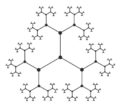
I.e., in the set of 5-adic numbers, 150 is closer to 25 than it is to 50. In this way, the entire geometry of the number line changes and numbers that intuitively appear far apart from each other can become close neighbours. One consequence is that p-adic number systems behave less like a line and more like a branching tree. While this viewpoint seems counterintuitive at first, it has far-reaching consequences and leads to interesting properties and applications. For instance, in p-adic spaces, geometry obeys a stronger version of the triangle inequality, known as the ultrametric property [2], which we shall explore in more detail in an upcoming follow-up article.
Some of these sequences do not converge to rational numbers, and the result is an entirely new number system called the p-adic numbers, usually denoted by Qₚ. Unlike the real numbers, there is not just one such system, but every prime number can generate its own p-adic “universe”, leading to an infinite family of number systems: 2-adic, 3-adic, 5-adic , … numbers. Each such family has its own geometry and topology, meaning that the tree-like structure looks different for each p-adic family. Remarkably, a theorem due to Ostrowski shows that, apart from the usual real numbers, these p-adic number systems are the only other possible way to complete the rationals.[2] In this sense, the rationals can be considered as the common “backbone”, shared by the real and the p-adic numbers. Beyond the rationals, no numbers are shared between the reals and the p-adic numbers, e.g., there is no p-adic equivalent for irrational numbers like pi.
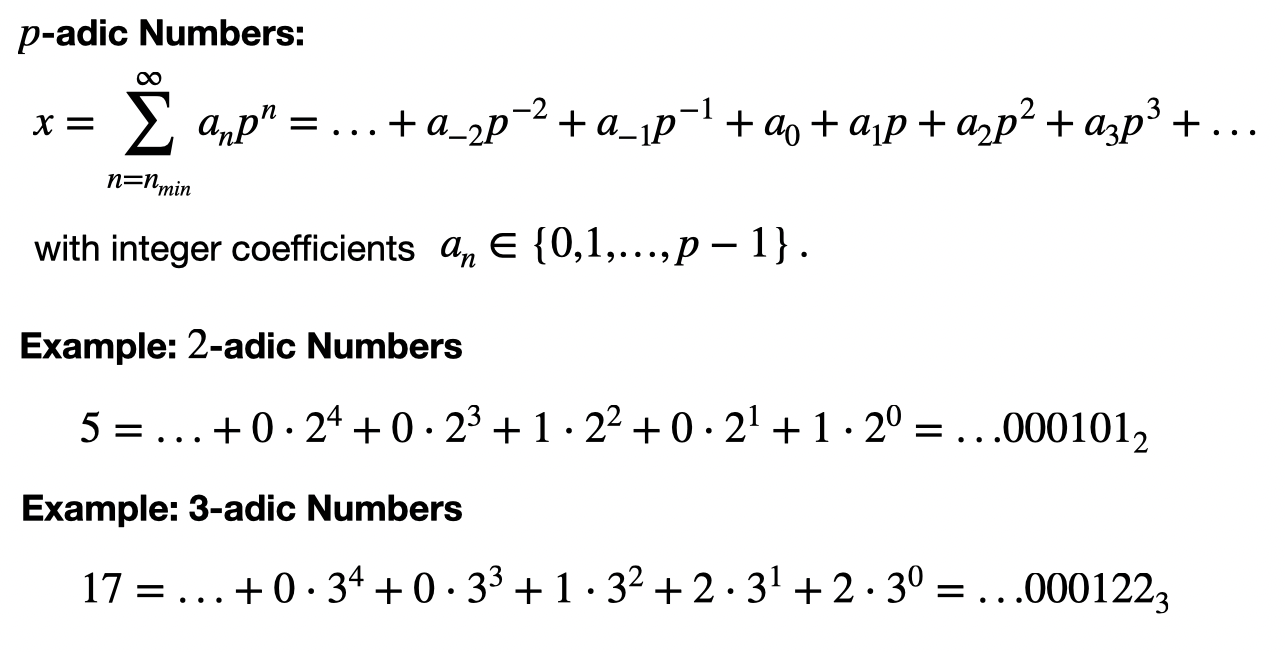
A natural question that arises is then: how can we explicitly represent any given p-adic number? The answer to this question is actually fascinatingly counterintuitive. Remember that the real numbers are often written as decimal expansions extending endlessly to the right of the decimal point, for instance 3.14159265… p-adic numbers behave almost in the opposite way: Instead of extending infinitely to the right of the decimal point, they can be written as expansions in powers of the chosen prime, that extend infinitely to the left of the decimal point, as shown below.
\( \normalsize x = \sum_{n=n_\text{min}}^\infty a_np^n =\ldots + a_{-2}p^{-2}+ a_{-1}p^{-1} + a_0 + a_1p + a_2p^2 + a_3p^3 +\ldots \)
Note that the indices n are integers that can be negative, whereas the coefficients an are integers such that
\( \huge 0 \leq a_n \leq p-1 \)
This structure implies that the expansion is infinite to the left, including increasingly negative powers of p, whereas it terminates after a finite number of non-zero terms to the right.
Although the notation may initially look unfamiliar, it turns out to be extremely powerful. For example, in the 2-adic world, numbers are naturally expressed using powers of 2. The image below demonstrates how to write down such a p-adic expansion:
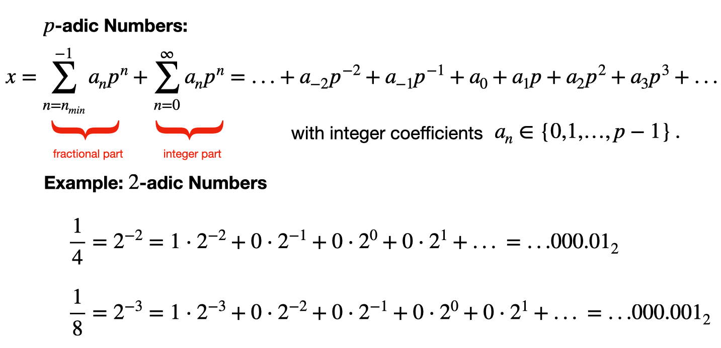
So far, we have only considered the p-adic expansions of integers, which contain only non-negative powers of p. However, every rational number, even fractions, can also be represented as a p-adic number. The only difference is that, just as ordinary decimal expansions of fractions require negative powers of 10 (e.g., 0.25=0.25=2×10⁻¹+5×10⁻²), p-adic expansions of fractions or negative numbers may also contain finitely many negative powers of p. The expansion then continues infinitely in the positive powers of p, we will see an example in a moment. In terms of the notation, this means that decimal expansions of real numbers may have finitely many digits to the right of the decimal point, whereas p-adic expansions may have finitely many digits to the right of the p-adic point but can extend infinitely to the left.
As mentioned, we can even represent negative integers and fractions with infinitely many non-zero digits in their p-adic expansions. The procedure for finding these expansions is surprisingly similar to the familiar long-division algorithm: we determine the coefficients one by one while ensuring, at each step, that the remaining part is divisible by a higher power of p. In the 2-adic expansion of -1, this process will always produce coefficients an =1, resulting in the following expansion:
\( \LARGE -1 = 1+2+2^2+2^3+2^4+\ldots = \ldots11111_2 \)
This result may seem very counterintuitive! For a more detailed explanation, see for example this video. Using the same reasoning, we can also find the p-adic expansions of fractions whose denominator is not a power of p. Such expressions are typically infinite and involve non-negative powers of p. In terms of 2-adic numbers, the fraction 1/3 , for instance, is represented by an infinite expansion extending to the left of the decimal:
\( \LARGE \frac{1}{3} = 1+2+2^3+2^5+2^7+\ldots = \ldots101011_2 \)
To conclude this introductory article, I would like to mention that p-adic numbers are not merely a mathematical curiosity but they surprisingly play an important role in various fields of modern mathematics. This is because certain problems become easier to understand when viewed through a p-adic lens. Examples of this can be found, for instance, in the context of cryptography or computer science, as the 2-adic numbers naturally represent binary notation. (For instance, the example in figure 4 illustrates that the 2-adic expansion of 5 is exactly its binary expansion, but with an infinite number of zeros extending to the left.) Moreover, over the last decades, ideas related to p-adic numbers and ultrametric spaces have also found applications in theoretical physics, including string theory and models of complex systems. Some of these applications will be discussed more in depth in our upcoming article.
References:
[1] Brekke, L., & Freund, P. G. (1993). p-Adic numbers in physics. Physics Reports, 233(1), 1-66.
[2] Rammal, R., Toulouse, G., & Virasoro, M. A. (1986). Ultrametricity for physicists. Reviews of Modern Physics, 58(3), 765.