How symmetries dictate physics

Figure 1. A phase transition.Ice changing into water is one example of a phase transition. It is near such phase transition that conformal symmetries play a crucial role. Image: PXFuel.

Correlation functions

In physics, one of the most useful types of quantities that we can compute are “correlation functions”.  These are formulas that encode how two random variables (that we consider to be building blocks of a quantum field theory in this context) are interconnected. A simple example can be found in iron. The correlation function between two random points in a chunk of iron will tell you how likely it is that two atoms at these points are magnetically oriented in the same direction. This is a function of the distance between the two atoms. Similar correlation functions exist for any numbers of points, and in the iron example such an ‘n-point correlation function’ express the likelihood that n atoms are all aligned.

Computing correlation functions can be highly non-trivial. When we are considering free theories (without interaction) or weakly-coupled ones, there is a whole machinery that has been developed over the last century to compute such quantities, but all these standard techniques fail for systems where the interaction between the building blocks is strong. Many of the most interesting physical phenomena lie in the realm of strongly-coupled quantum field theories and this is why finding new tools to shed light on these systems is a pressing issue.  Amongst the set of new ideas, the conformal bootstrap is one of the most promising. Let me explain how this came about by introducing phase transitions.

Phase transitions

It is a well-known fact that many systems can experience phase transitions when we vary some of their parameters. The prototypical example is water, which has three obvious phases that depend on the temperature and the pressure of the system. At atmospheric pressure, we can easily experience the water phase transition from solid to liquid around zero degrees Celsius. Many other systems experience such phase transitions. The different phases of a system, and how these phases depend on the parameters, can be nicely depicted in a so-called phase diagram. For example, figure 2 below shows the phase diagram for water. In the phase diagram of every fluid, there exist critical points, which are specific points beyond which there is no sharp distinction between the liquid and the gas phases. This is because at these points, the fluid is so hot and compressed that the distinction between the two phases is almost non-existent.

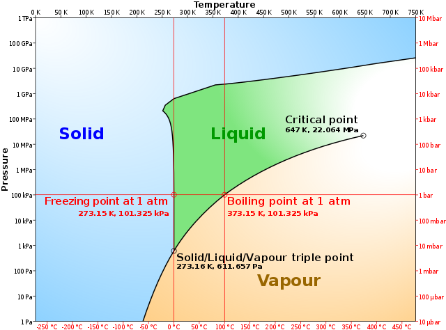
Figure 2. Phase diagram of water.Image: Cmglee.

These critical points are special, and they have one particularly useful universal property. Close to them, the correlation functions between two points do not  decay exponentially with the distance d, as one could expect from general mathematical reasoning, but rather they obey power law decay. This means that the critical points can be characterized by the exponent α of a power law behaviour d^–α, which is called a critical exponent. These critical exponents are robust quantities that can be measured in the laboratory. Over the years, it came as shocking that actually, these critical exponents turn out to be the same for a wide class of extremely different systems. This very surprising, yet crucial phenomenon, goes under the name “universality”: all critical points that we know of fall into a small number of universality classes that have the same critical exponent. These classes are characterized by the symmetries of the system. This is because at long distance, microscopic details of the system do not matter and all theories with the same symmetry look the same near the critical point. There are many examples of this, but a famous one is iron at the critical temperature where the material is not magnetized anymore: its critical exponent is the same as the one that describes water at its critical point. This strongly hints at the fact that all instances of a universality class, even though they don’t share microscopic details, have to have something in common, and this common feature is their symmetry.

Conformal symmetry

All systems that are in the same universality class have the same symmetries. Such symmetries can be nicely encoded in an object that mathematicians call a ‘group’, the set of symmetry transformations that leave the system invariant. It was later realized that theories at a critical point share an enhanced symmetry which is called conformal symmetry. The conformal symmetry group consists of rotations, translations, rescaling and a particular set of transformations that preserve angles. The rescaling symmetry is crucial here, because it means that if you zoom in or out in a system that has conformal symmetry, you will see the exact same pattern, and there is thus no absolute notion of distance, or in other words: the system has no intrinsic scale.

This symmetry is obviously not a symmetry of the world we live in at large, but when present in so-called conformal systems, is extremely powerful. These systems are best described by a mathematical framework called conformal field theory. In this framework, conformal symmetry is extremely constraining and fixes the two-point and three-point correlation functions up to free numbers that are theory dependent.  In two dimensions, the symmetry even gets enhanced to an infinite dimensional ‘algebra’ (an algebra is another useful mathematical construct with in this case an infinite number of conserved quantities) which lies at the heart of the huge control we have over these theories. This was used in the 1980s to fully solve a simple two-dimensional model of spins called the Ising model using the bootstrap method that is the main topic of this article.

The bootstrap philosophy is the following: Use general principles as well as consistency conditions to infer what the correlation functions of the system you are studying can be. In the context of conformal field theories, it means that first, we need to understand the full consequences of conformal symmetry, as well as to impose further consistency conditions. In two dimensions, as already mentioned, this is enough to solve some lattice spin models exactly. In higher dimensions, the algebra is not infinite dimensional and there are far fewer conformal symmetries.  For these systems, despite the fact that the consistency conditions, which are called “bootstrap equations” were written a long time ago, they proved too hard to be solved back then and this direction was abandoned.

The conformal bootstrap

Let us delve a little bit deeper into the mathematical description of the bootstrap idea. A conformal field theory (CFT) can be described in abstract terms. It contains a possibly infinite number of local operators O(x₁) … O(x_n) which capture measurements of the system at a spacetime point x_i. As we already mentioned, conformal symmetry severely constrains the form of the two-point correlation function of these operators. Such two-point correlation functions are given by

This expression depends only on the distance x-y between the two operators, and Δ is a number called the conformal dimension that specifies how an operator changes when we zoom in or out. Thus, two-point correlation functions are fixed by the symmetry up to a single number. The power of conformal symmetry extends also to three-point correlators. For three operators in the theory, say O₁, O₂ and O₃, these must have the form

This might look complicated, but the crucial point is that (since the Δs are known from the 2-point functions) the only new unknown, for any CFT, is the number f₁₂₃, which is theory dependent and is called the three-point coefficient. At this point, one is finished: it turns out that to completely characterize a CFT, knowing the set of operators as well as their conformal dimensions and the three-point coefficient is sufficient. This is where the bootstrap equation comes in: solving it actually yields for you the set of consistent numbers that can give you a physically sensible theory.

Applying the bootstrap

In CFTs, there exists a sensible way to glue to glue three-point functions together to obtain higher-order correlation functions. You can trade a four-point function for a product of three-point functions provided you sum over all the operators that are allowed in the theory. Schematically, this is the statement that

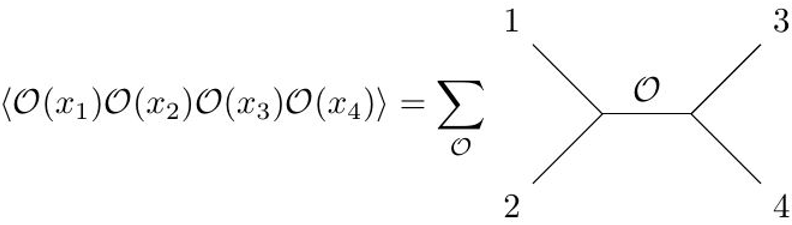
This is the essence of the “boostrap equation”, which is the statement that for the theory to be consistent, the order in which you do this should not matter. This implies that different ordering should be the same, or that

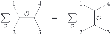
This equation non-trivially relates the conformal dimensions Δ of the operators of the theory, as well as the three-point function coefficients f₁₂₃. It involves an infinite number of term and must be satisfied for any arbitrary four positions 1, 2, 3, 4. This equation was known for a long time, but could be solved only in two-dimensions as we mentioned earlier.

The breakthrough happened in 2008. While trying to solve a seemingly unrelated problem, a group of physicists wrote down bootstrap equations that a CFT should have to get some peculiar properties that they were looking after. Their equation was too hard to solve exactly, and they thus decided to instead use it to put bounds on the allowed parameters of the theory. This idea happened to be revolutionary.

The key idea is the following: If you take the boostrap equation and put both terms on the same side of the equal sign, you get something that schematically looks like

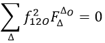
This equation implies that the sum of a positive quantity (because it is squared) times a vector should be zero. Such an equation is hard to solve exactly but it is easier to rule out forbidden configurations. Indeed, imagine four vectors that originate from a point. It they all point roughly in the same direction, as in the right figure below, it is impossible for multiples of them with positive coefficients to sum to zero – there is simply no ‘arrow pointing backwards’ to get back to zero – and you can thus rule out this configuration of vectors. More generally, if a plane can be found, such that all vectors point to one side of the plane, then there exists an imbalance and the configuration is not allowed, since it can not solve the bootstrap equation.

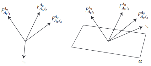
Figure 3. Configurations of vectors.The left configuration is allowed, as positive combinations can point to zero. The right configuration does not have this property. This image and the two diagrammatic formulas above are taken from The Conformal Bootstrap, D. Poland and D. Simmons-Duffin, Nature Physics 12 2016.

This technique has now been used in a wide range of two- and three-dimensional conformal field theories with great success. It yielded the most precise determination of the critical exponents of many of these theories, and excluded a big part of parameter space.

In addition, CFTs are now considered as the building blocks of all quantum field theories. Quantum field theory (QFT) is the language of modern theoretical physics, and allows to describe an extremely big number of widely different phenomena. Physicists have discovered that any QFT can be seen as a deformed CFT. Thus, uncovering their theory space (the space of allowed CFTs) is a first step towards the complete classification of quantum field theories, including the strongly-coupled ones that have been so difficult to describe.

Finally, through the AdS/CFT correspondence, the conformal bootstrap becomes a powerful tool to investigate quantum gravity. AdS/CFT relates a CFT living on the boundary of a higher-dimensional spacetime to a theory of quantum gravity inside of that spacetime. We can thus see any CFT has giving rise or ‘sourcing’ a quantum theory of gravity. Using the bootstrap, it is now believed that we know what the necessary and sufficient conditions are that a CFT must satisfy in order to reproduce general relativity in the bulk of AdS (i.e. ‘negatively curved’) spacetime. Though our universe does not appear to be AdS, the AdS/CFT correspondence combined with the bootstrap program has already shed light on many conceptual issues that arise when trying to understand gravity at the quantum level. The hope is that by pursuing this program, we will understand the general organizing principle lying beyond what we experience.