Quantum Doodles

Pool balls and electrons

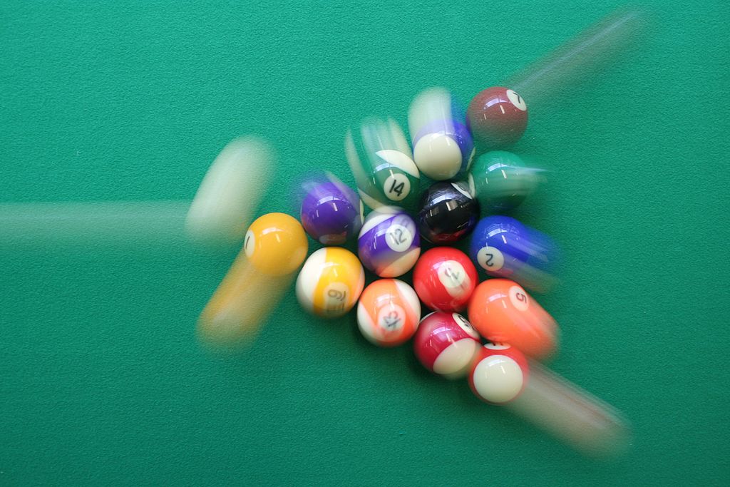
Imagine two pool balls coming at each other head-on. What will happen? They will collide and bounce off each other; nothing spectacular. But what happens if we replace the balls with electrons? Surely something similar must occur, right? As they come closer the electromagnetic force between the electrons will repel both of them back into the directions they were coming from. If you are an ordinary person, like me, this would have been as far as your imagination would have got. This was certainly not the case for Richard Feynman.

Richard Feynman was a bongo-playing, down-to-earth (though certainly not flawless), theoretical physicist known for his great contributions to quantum theory. Feynman imagined the electron differently than we usually do. He imagined the electron doing all sorts of things along its trajectory: things like moving on weird paths or emitting and re-absorbing photons at every step of its way. He did not see the ‘pool ball collision’ analogy for electrons; rather Feynman imagined the electrons, as they approached each other, exchanging photons. By the law of conservation of momentum via the photon exchange, they would repel each other.  This would explain the electromagnetic force that pushes both electrons apart and the force we are all familiar with in a natural way; but that was not all that Feynman imagined the quantum world would look like.

One layer deeper, he saw that the emitted photons also behaved in ways we usually do not encounter. The photons emitted by the electrons would destroy themselves along their path leaving behind an electron and an anti-electron (a positron), which then would recombine into the original photon.

One layer deeper still, Feynman saw that these ‘internal’ electrons and anti-electrons, in their short lifetime, would also do the same as the initial electrons. And so on…

Virtual particles and Feynman diagrams

These intermediate particles that appear in the scattering process of the two electrons are called virtual particles. The name comes from the fact that we cannot measure them, as they are exactly the particles that exist in between scattering processes – and we need such processes to do a measurement to begin with! To express these virtual particles mathematically is really difficult. Just to scare you: this is the expression used for the process of just one photon being exchanged in the scattering process:

\( \mathcal{M} = \Big( -q \, \bar{e}^-(p_1′)\, \gamma^\mu \, e^-(p_1)  \Big) \cdot  \left[ \frac{-g_{\mu \nu}}{k^2}\right] \cdot \Big( -q \, \bar{e}^-(p_2′)\, \gamma^\mu \, e^-(p_2)  \Big) \).

\( \mathcal{M} \) roughly gives you the probability that this specific scattering process happens. Don’t lose too much time in understanding the symbols. The only fact I want to convey is that these expressions get hard very fast!

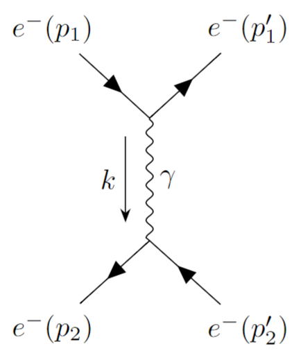
Given that it would be inhuman to compute with these mathematical expressions for processes of multiple virtual particles, we have to thank Feynman for his incredible creativity. He developed a way to represent these processes in terms of diagrams: the famous Feynman diagrams. The equation above reduces to this simple drawing:

Isn’t this nice? Physicists study hard for multiple years to understand the intricacies of quantum theory, just to end up at toddlers’ doodles.

Instead of trying to understand all the mathematics, let’s try to find the dictionary¹ relating individual parts of the equation with the Feynman diagram. You can see that the equation is made out of two building blocks:

• Twice we find the expression \( -q \, \bar{e}^-\, \gamma^\mu \, e^-  \), which we call the electron current  
• Once we have \( -g_{\mu \nu}/k^2 \), which we call the photon propagator. The photon is the carrier of the electromagnetic force and hence we see that the lines in between two general currents always gives the interaction/force between two particles.

We now identify these expression with the Feynman diagram:

• The currents are the straight lines. These describe the electrons flowing in and out of the scattering process. One detail, that is important, is the fact that there is the constant \( q \) appearing in the current. This is the electric charge of the electron, which in general is referred to as the coupling constant. One always multiplies \( q \) whenever a straight line meets a wavy line. In our diagram above we find two of these vertices, hence we have \( q^2 \) in our expression for the probability. Keep this in mind for the next section!
• The photon propagator is illustrated via wavy lines between the two electron currents. This precisely describes the fact that one electron sends out a photon and pushes the other electron away, thereby resulting in the scattering of electrons.

With this knowledge we can now begin to draw as many Feynman diagrams as we like and see what physics (and mathematics) comes out of it².

Ad infinitum³

In principle, to get the full scattering probability we would need to add more and more diagrams, as we consider all possible things that could happen. A full scattering probability is important as one will want to eventually confirm, via measurements, whether a given theory describing the scattering process matches our real world. In other words: this allows us to see how the ’pool ball electrons’ actually collide.

But how can we possibly compute anything at all, if we add an infinite amount of these diagrams? This would look like something like this:

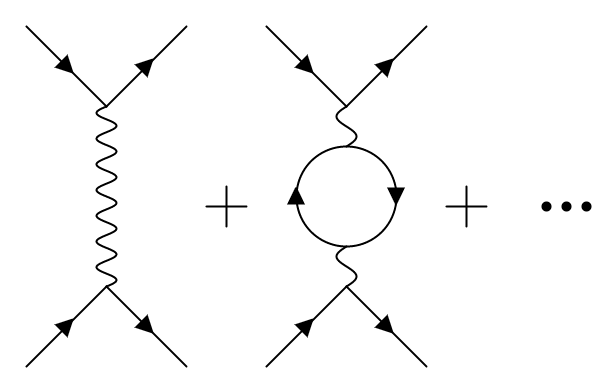
Well, the subtlety comes from the fact that we have the coupling constant \( q \) in our expressions! It turns out that this number is very small, meaning \( e \ll 1 \), and hence if we take higher powers of it we arrive at smaller and smaller numerical values⁴. Now back to the diagrams: one can see that the more complicated the diagrams get, the more vertices they acquire and therefore the more powers of the coupling constant we need to multiply. This results in the fact that weird and crazy long diagrams come with extremely small prefactors, and so we would expect them to hardly contribute to the probability of the process. Hence we usually only focus on the first couple of them!

Usually we call the first diagram the classical contribution, as it describes what we expect classically, namely the electromagnetic repulsion, and then the rest we address as quantum corrections, because of the fact that these are processes that do not happen in the classical model of electrodynamics.

Recap and looking ahead

Important things to remember are:

1. Quantum mechanically, in a scattering process, there are an infinite amount of possible things happening. For electron scattering, one can keep track of the complexity of the process by the power of the coupling constant \( q \).
2. There are two ways of describing a scattering process: either by a long mathematical expression or by drawing the famous Feynman diagrams. Feynman diagrams, therefore, allow us to see what the interaction between two particles is for any theory, even for gravity – though we shall see that for that force, there are many additional subtleties and unsolved problems!
3. We need to sum over multiple Feynman diagrams to get the full probability. The more diagrams we add, the more quantum corrections we take into account.

This is only the beginning of our story. In String Gravity à la Feynman: Part 2  we shall see the astonishing connection between gravity and geometry that Einstein found in 1915. In String Gravity à la Feynman: Part 3 we then see how string interactions are also describable via Feynman diagrams, and that the resulting geometry of that scattering process will lead to the fact that string theory is a theory of quantum gravity.

^[1] For further reference we call this dictionary the Feynman rules of any given theory.
^[2] Of course I simplified a bit here and swept a lot of mathematical details under a big rug. But the idea that we can draw diagrams and find mathematical expressions from these drawings is exact! In 1965, Feynman was awarded the Nobel Prize in Physics precisely because of these ”deep-ploughing consequences for the physics of elementary particles”.
^[3] In Latin this means ‘without ever coming to an end’.
^[4] For instance if \(q=0.1\) then \(q^2=0.01\) and \(q^3=0.001\), and so on.